Optimizing heavy models with early exit branches
Everyday models get heavier and heavier (in terms of learnable parameters). For example, LEMON_large has 200M parameters and GPT-3 has over 175 billion parameters!

Though they give State-of-the-Art Performance, how well are they deployed today? This calls for an efficient and faster method for training and inferring. So, we explore various methods through which we can speed up compute-intensive networks while preserving accuracy!
This blog will cover 2 papers:
- Fei, Zhengcong, et al. “DeeCap: Dynamic Early Exiting for Efficient Image Captioning.” Proceedings of the IEEE/CVF Conference on Computer Vision and Pattern Recognition. 2022. [paper link]
- Wołczyk, M., Wójcik, B., Bałazy, K., Podolak, I. T., Tabor, J., Śmieja, M., & Trzcinski, T. (2021). Zero Time Waste: Recycling Predictions in Early Exit Neural Networks. Advances in Neural Information Processing Systems, 34, 2516–2528. [paper link]
Individual blog posts explaining these papers are given below as well:
First, we cover “DeeCap: Dynamic Early Exiting for Efficient Image Captioning”:
Early Exiting for Image Captioning Models

But first, — WHAT IS EARLY EXITING?
As described in this paper as “BranchyNet”, these neural networks have exit branches at specific locations throughout the network.
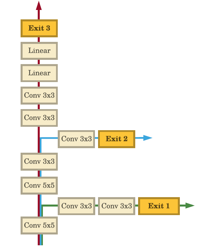
Source: https://arxiv.org/pdf/1709.01686v1.pdf
What’s the main idea of these branches then?
Suppose you have 100 layers in a neural network. After passing the input image through the input layer, it must go through all layers to generate an output. But, you realize that for some samples, you can classify them accurately after just passing through some n layers (for example, 5 layers). In this case, feed-forward passes through all other layers is wasteful in terms of computational resources. So, we exit at the nth layer through a branch.
This is especially useful in large networks that have 100s of layers in them.
It even allows large networks like AlexNet to be deployed for real-time inferences. But when it comes to Image captioning models, there’s a catch.
Image Captioning Models
Image captioning models are different. They are basically **Encoder-Decoder models — **I won’t go deep into the Encoder-Decoder architecture, but on the surface level, the encoder part creates a representation/intermediate vector based on the input, and the decoder predicts the token(word) at each timestep.
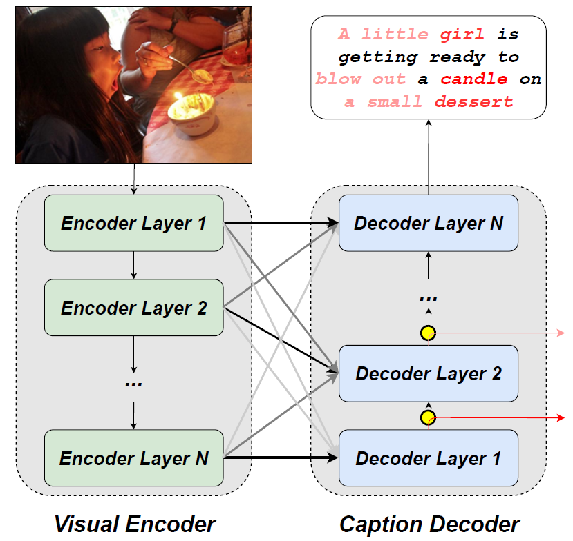
Speaking of these encoder-decoder models, can we also apply early-exit branches to them? Yes, but with some modifications.
These “modifications” are made possible, thanks to Fei, Zhengcong, et al. and their research work “DeeCap: Dynamic Early Exiting for Efficient Image Captioning”.
In this paper, the authors saw that conventional early exiting is not possible in the case of encoder-decoder networks, since at the shallow level, the representations generated by the decoder layers are insufficient to predict tokens accurately, since they lack high-level semantic information.
That is, let’s say that we are early exiting after n decoder layers. The representation produced by those n decoders is not sufficient to predict accurately, and we still need the outputs from the deeper decoder layers after them.
The workaround? Try to replicate the outputs of the deeper decoder layers!
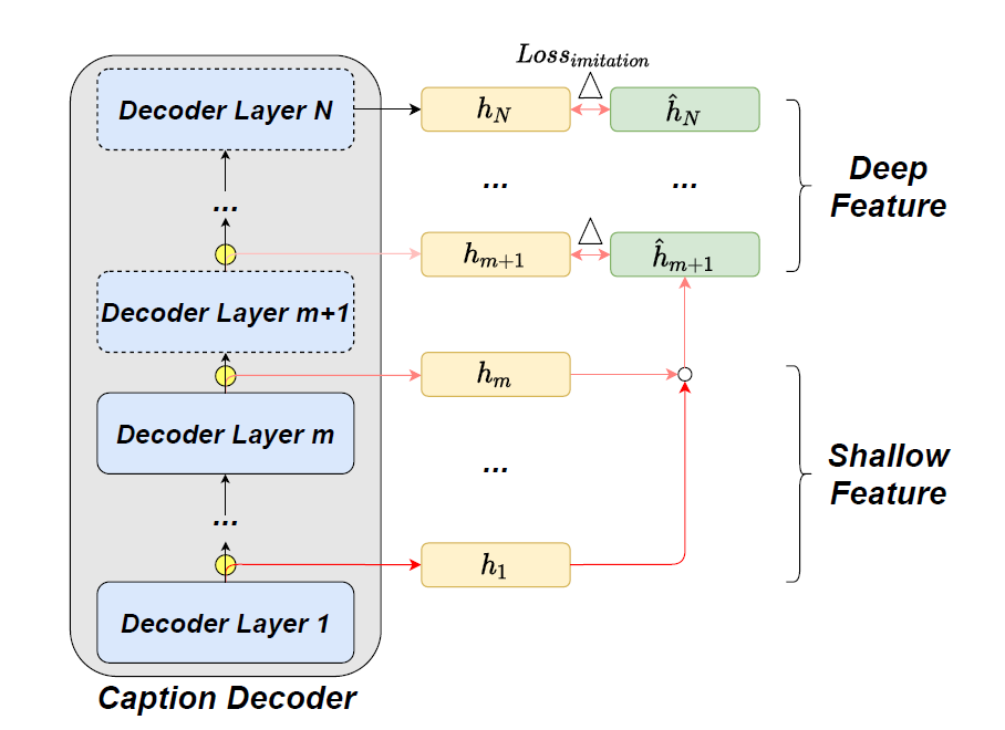
First, let us assume that we are going to exit early at layer m. So this means that for layer ‘k’, where k≤m we have done the forward pass. And for every layer ‘k’ where k>m, we have to replicate the representations.
This replication is done with the help of imitation learning. Let’s say we want to replicate the representation of layer k where k>m. The k-th imitation network paired with the k-th layer inputs the truly hidden state h_m and outputs:
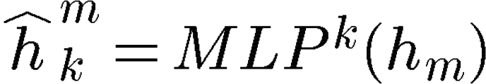
Imitated Representation
where MLP is a multi-layer perception. But these MLPs also need to be trained accordingly, so that they can output the imitation representations. This is done with the help of cosine similarity as our main loss function.
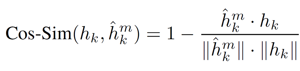
Cosine Similarity Loss Function
Now, we found a way to get the output of the deeper decoder layers using imitation learning, and how to train the MLP that facilitates imitation learning.
But we are still a few steps away from achieving early-exiting. Now that we have the representations of all the decoder layers, we can group them into 2 kinds: h-shallow are the layers that performed the actual feed-forward, and h-deep are the layers that used imitation layers.
Now, we need to aggregate these h-shallow and h-deep layers. This aggregation is done with the help of a fusion strategy. There different fusion strategies that we can use are:
- Average Strategy
- Concatenation Strategy
- Attention-Pooling Strategy
- Sequential Strategy
Now that we finished aggregating the h-shallow layers separately, and h-deep layers separately, we now need to know how to merge them.
This calls for a Gate Decision Mechanism.
So far we know these facts:
- h-deep layers representations are produced using imitation networks.
- h-shallow layers representations are produced by the actual feed-forward mechanism.
Since the h-shallow layers have actually seen the input data, they are more likely to be reliable. So, we need to find a balance factor to control how much information we need from h-shallow vs h-deep. This balance factor α is calculated using the following formula:
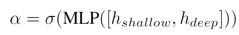
With this balancing factor, we can finally represent the final merged information as
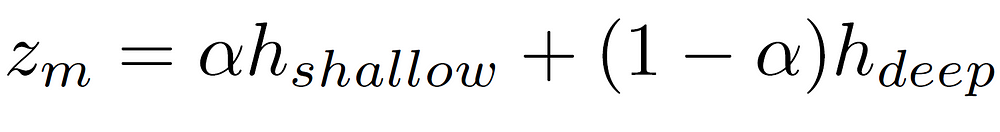
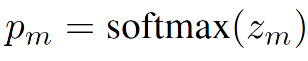
After applying the softmax function to zₘ, we can calculate the output class distribution as
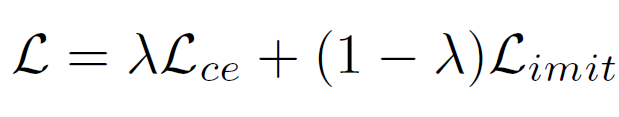
But, we also need to dynamically learn the balancing factor. The corresponding loss function is:
Thus, the final training objective is:

Now, we can finally talk about training and inference!
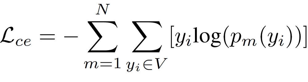
Remember that we calculated pₘ previously? By calculating the entropy of pₘ as H(pₘ), we calculate the prediction confidence of the current token at layer m. We then compare the prediction confidence with a manually selected threshold τ. Once this value is lower than the threshold, we can exit!
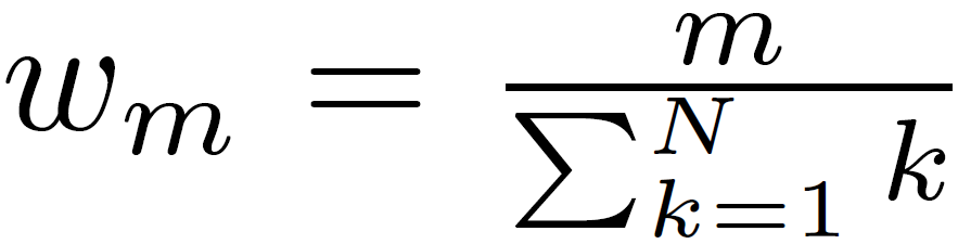
Also, note that the shallow layer’s weights will be updated more frequently because they are receiving more update signals than the deep layers. So, while calculating the cross entropy loss of each layer, we reweight them using the following equation:
Added to this, the authors argue that updating all parameters at the same time at each time step will damage the well-trained features during fine-tuning. Therefore, they try to freeze the parameters at each layer with a probability p, and it linearly decreases from 1 to 0 with depth.
And that’s how we add anearly exit to encoder-decoder-based models!
Next, we look into another application of early-exit network, where we try to go green by recycling predictions! (“Zero Time Waste: Recycling Predictions in Early Exit Neural Networks”)
Going green by recycling predictions!
According to this research, training a single deep-learning model can generate up to 626,155 pounds of CO2 emissions — that’s roughly equal to the total lifetime carbon footprint of five cars! And not to mention that usually, deep learning models are run several times while trying to predict a value, i.e. during INFERENCE!
But, is there a way to reduce the carbon footprint of the inference process? In this blog post, we saw can actually skip some layers during inference and still achieve SoTA-level accuracy. But, did you also notice we also did less number of computations?
According to Wołczyk, Maciej, et al. in this paper, we can further reduce the number of computations — while also increasing the accuracy!
The Argument:
This paper makes an important argument that while trying to exit early in a Convolutional Neural Network, sometimes we discard the output if it is below a threshold, but those discarded outputs may contain useful information.
Thus, we can recycle those discarded outputs to feed the internal classifier in the next early exit branch with useful information.
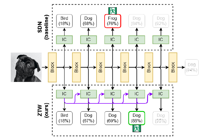
Network Overview. Source: https://arxiv.org/abs/2106.05409
This is done with the help of cascade connections! The concept of cascading is to keep stacking up the information from the previous ICs, as we go deeper!
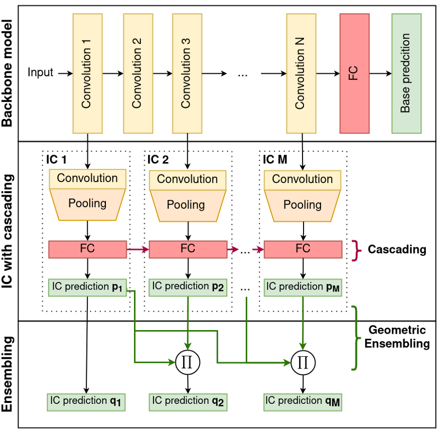
Network Architecture. Source: https://arxiv.org/abs/2106.05409
We know that at each branch connection, we have an Internal Classifier that takes care of the feed-forward. After applying the softmax function to these ICs, we can get the probabilities of each class. This is given by the formula:

where g_ϕm is the mᵗʰ IC’s output and f_θm is the output from the hidden layer m in the backbone model. That is, we receive information from both the actual backbone model and the previous IC — thus capturing the information that the previous IC learned too.
Are we done yet?

Almost there!
There is one more way in which we can recycle our predictions — the predictions themselves!
In the final stage of this model, they use ensembling to combine the previous predictions. This is represented by the formula:
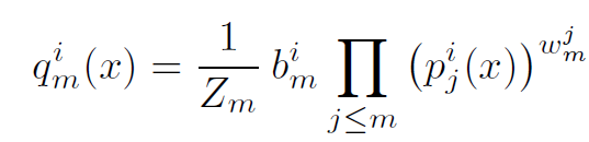
Probability of each output class
Where pⱼ is the output of ICs, bₘ, and wₘ are trainable parameters, and Zₘ makes sure that the sum of qₘ for all classes is equal to 1. ‘i’ represents the iᵗʰ class and j represent the layers up to current layer m.
Once qₘ is greater than a particular threshold for any class i, we can output the prediction, and thus exit early! Else, we feed it forward to the next IC, and continue the computation.
Overview of this approach
This approach does the following workarounds:
- First, we feed forward the logits of the current Internal Classifier to the next Internal Classifier
- Next, we can aggregate/ensemble the previous IC’s prediction by using the above formula

The end!
Also, look into my friend’s blog on “Optimizing Compute-Intensive Models using Model Pruning”
References:
- Fei, Zhengcong, et al. “DeeCap: Dynamic Early Exiting for Efficient Image Captioning.” Proceedings of the IEEE/CVF Conference on Computer Vision and Pattern Recognition. 2022.
- Teerapittayanon, Surat, Bradley McDanel, and Hsiang-Tsung Kung. “Branchynet: Fast inference via early exiting from deep neural networks.” 2016 23rd International Conference on Pattern Recognition (ICPR). IEEE, 2016.
- Strubell, E., Ganesh, A., & McCallum, A. (2019). Energy and policy considerations for deep learning in NLP. arXiv preprint arXiv:1906.02243.
- Wołczyk, M., Wójcik, B., Bałazy, K., Podolak, I. T., Tabor, J., Śmieja, M., & Trzcinski, T. (2021). Zero Time Waste: Recycling Predictions in Early Exit Neural Networks. Advances in Neural Information Processing Systems, 34, 2516–2528.