Going green by recycling predictions!

According to this research, training a single deep-learning model can generate up to 626,155 pounds of CO2 emissions — that’s roughly equal to the total lifetime carbon footprint of five cars! And not to mention that usually, deep learning models are run several times while trying to predict a value, i.e. during INFERENCE!

But, is there a way to reduce the carbon footprint of the inference process? In this blog post, we saw can actually skip some layers during inference and still achieve SoTA-level accuracy. But, did you also notice we also did less number of computations?

According to Wołczyk, Maciej, et al. in this paper, we can further reduce the number of computations — while also increasing the accuracy!

The Argument:

This paper makes an important argument that while trying to exit early in a Convolutional Neural Network, sometimes we discard the output if it is below a threshold, but those discarded outputs may contain useful information.

Thus, we can recycle those discarded outputs to feed the internal classifier in the next early exit branch with useful information.

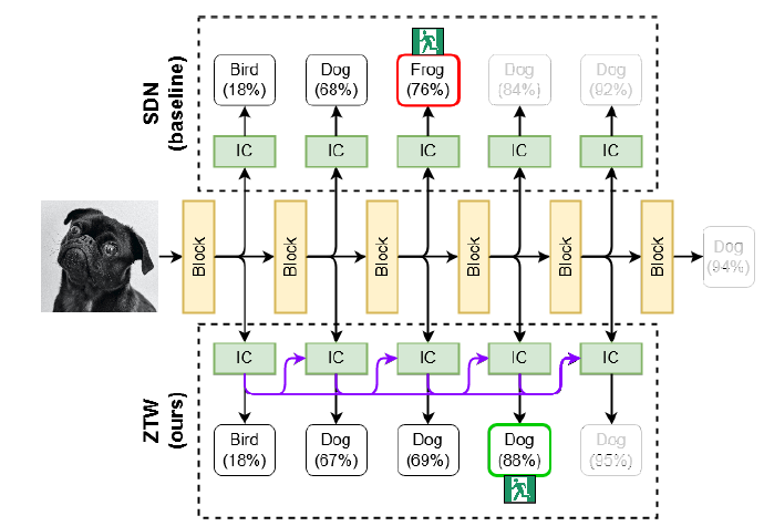
Network Overview. Source: https://arxiv.org/abs/2106.05409

This is done with the help of cascade connections! The concept of cascading is to keep stacking up the information from the previous ICs, as we go deeper!

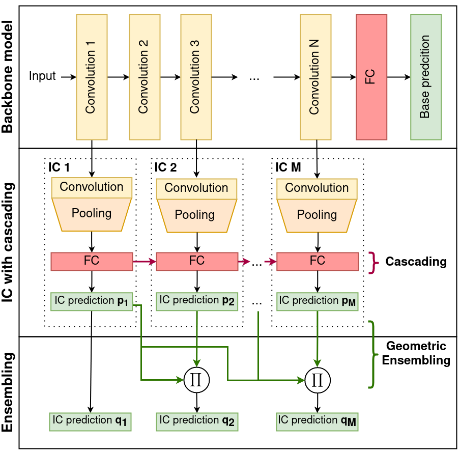
Network Architecture. Source: https://arxiv.org/abs/2106.05409

We know that at each branch connection, we have an Internal Classifier that takes care of the feed-forward. After applying the softmax function to these ICs, we can get the probabilities of each class. This is given by the formula:

where g_ϕm is the mᵗʰ IC’s output and f_θm is the output from the hidden layer m in the backbone model. That is, we receive information from both the actual backbone model and the previous IC — thus capturing the information that the previous IC learned too.

Are we done yet?

Almost there!

There is one more way in which we can recycle our predictions — the predictions themselves!

In the final stage of this model, they use ensembling to combine the previous predictions. This is represented by the formula:

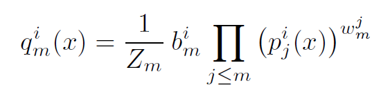
Probability of each output class

Where pⱼ is the output of ICs, bₘ, and wₘ are trainable parameters, and Zₘ makes sure that the sum of qₘ for all classes is equal to 1. ‘i’ represents the iᵗʰ class and j represent the layers up to current layer m.

Once qₘ is greater than a particular threshold for any class i, we can output the prediction, and thus exit early! Else, we feed it forward to the next IC, and continue the computation.

Conclusion:

This approach does the following workarounds:

1. First, we feed forward the logits of the current Internal Classifier to the next Internal Classifier
2. Next, we can aggregate/ensemble the previous IC’s prediction by using the above formula

The end!

References:

1. Strubell, E., Ganesh, A., & McCallum, A. (2019). Energy and policy considerations for deep learning in NLP. arXiv preprint arXiv:1906.02243.
2. Wołczyk, M., Wójcik, B., Bałazy, K., Podolak, I. T., Tabor, J., Śmieja, M., & Trzcinski, T. (2021). Zero Time Waste: Recycling Predictions in Early Exit Neural Networks. Advances in Neural Information Processing Systems, 34, 2516–2528.